Chapter 6 Escaping from Mars

Suppose you landed on Mars by mistake and you want to leave that rocky planet and return home. To escape from a planet you need a very important piece of information: the escaping velocity from the planet.

What on Mars is the escape velocity?

We are going to use the same experiment that Newton thought when thinking about escaping from the gravity of Earth. Gravity pulls us down, so if we shoot a cannonball, as in the sketch shown below, what will happen? For some velocities, the cannonball will return to Earth, but there’s a velocity at which it scapes since the gravitational pull is not enough to bring it back to the surface. That velocity is called escape velocity.

begin 
  using Images
  using Plots
    im_0 = load("./06_gravity/images/cannonball_.png")
    plot(im_0)
    #img_small = imresize(im_0, ratio=1/3)

end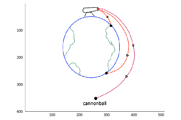

To simplify, we approximate the escape velocity as:

\(v_{escape}=\sqrt{2*g_{planet}*r_{planet}}\)

where \(r\) is the radius of the planet and \(g\) the constant of gravity at the surface. Suppose that we remember from school that the velocity of scape from Earth is \(11\frac{km}{s}\) and that the radius of Mars if half of the earth’s.

We remember that the gravity of Earth at its surface is \(9.8\frac{m}{s^2}\), so all we need to estimate the escape velocity of Mars is the gravity of the planet at its surface. So we decide to make an experiment and gather some data. But what exactly do you need to measure? Let’s see.

We are going to calculate the constant \(g_{mars}\) just throwing stones. We are going to explain a bit the equations regarding the experiment. The topic we need to revisit is Proyectile Motion.

## Proyectile Motion

Gravity pulls us down to Earth, or in our case, to Mars. This means that we have an acceletation, since there is a force. Recalling the newton equation:

\(\overrightarrow{F} = m * \overrightarrow{a}\) where \(m\) is the mass of the object, \(\overrightarrow{F}\) is the force(it’s what make us fall) and \(\overrightarrow{a}\) is the acceleration, in our case is what we call gravity \(\overrightarrow{g}\). The arrow \(\overrightarrow{}\) over the letter means that the quantity have a direction in space, in our case, gravity is pointing to the center of the Earth, or Mars.

How can we derive the motion of the stones with that equation?

In the figure below we show a sketch of the problem: We have the 2 axis, \(x\) and \(y\), the \(x\) normally is parallel to the ground and the \(y\) axis is perpendicular, pointing to the sky. We also draw the initial velocity \(v_0\) of the proyectile, and the angle \(\theta\) with respect to the ground. Also it’s important to notice that the gravity points in the opposite direction of the \(y\) axis.

begin 
    im_1 = load("./06_gravity/images/trajectory.png")
    plot(im_1)
end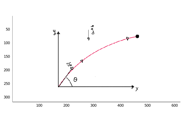

But what are the trayectory of the proyectile? and how the coordinates \(x\) and \(y\) evolve with time?

If we remember from school, the equations of \(x\) and \(y\) over time is:

\(x(t) = v_0*t*cos(θ)\)

\(y(t) = v_0*t*sin(θ) -\frac{g*t^2}{2}\) where \(t\) is the time at which we want to know the coordinates.

What the equations tell us?

If we see the evolution of the projectile in the \(x\) axis only, it follows a straight line (until it hits the ground) and in the \(y\) axis the movement follows a parabola, but how we interpret that?

We can imagine what happens if we trow a stone to the sky: the stone starts to go up and then, at some point, it reaches the highest position it can go. Then, the stone starts to go down.

How does the velocity evolve in this trajectory?

Since the begining, the velocity starts decreasing until it has the value of 0 at the highest point, where the stone stops for a moment, then it changes its direction and start to increase again, pointing towards the ground. Ploting the evolution of the height of the stone, we obtain the plot shown below. We see that, at the begining the stone starts to go up fast and then it slows down. We see that for each value of \(y\) there are 2 values of \(t\) that satisfies the equation, thats because the stone pass twice for each point, except for the highest value of \(y\).

begin 
    im_3 = load("./06_gravity/images/img90_.png")
    plot(im_3)
end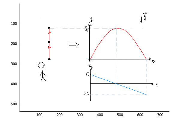

So, in the example we ahve just explained, we have that the throwing angle is θ=90°, so sin(90°)=1, the trajectory in \(y\) becomes:

\(y(t) = v_0*t -\frac{g*t^2}{2}\) And the velocity, which is the derivative of the above equation becomes: \(v_{y}(t) = v_{0} -g*t\)

Those two equations are the ones plotted in the previous sketch, a parabola and a straight line that decreases with time. It’s worth to notice that at each value \(y\) of the trajectory, the velocity could have 2 values, just differing in its sign, meaning it can has 2 directions, but with the same magnitude. So keep in mind that when you throw an object to the sky, when it returns to you, the velocity will be the same with the one you threw it.

6.1 Calculating the constant g of Mars

Now that we have understood the equations we will work with, we ask:

how do we set the experiment and what do we need to measure?

The experiment set up will go like this: - One person will be throwing stones with an angle. - The other person will be far, watching from some distance, measuring the time since the other throw the stone and it hits the ground. The other measurement we will need is the distance Δx the stone travelled. - Also, for the first iteration of the experiment, suppose we only keep the measurements with and initial angle θ~45° (we will loosen this constrain in a bit).

begin 
    im = load("./06_gravity/images/sketch_2.png")
    plot(im)
end

Suppose we did the experiment and we have measured then the 5 points, Δx and Δt, shown below:

Δx_measured = [25.94, 38.84, 52.81, 45.54, 17.24]

## 5-element Array{Float64,1}:
##  25.94
##  38.84
##  52.81
##  45.54
##  17.24

t_measured = [3.91, 4.57, 5.43, 4.85, 3.15]

## 5-element Array{Float64,1}:
##  3.91
##  4.57
##  5.43
##  4.85
##  3.15

Now, how we estimate the constant g from those points?

Using the equations of the trajectory, when the stone hits the ground, y(t) = 0, since we take the start of the \(y\) coordinate in the ground (negleting the initial height with respect to the maximum height), so finding the other then the initial point that fulfill this equation, we find that:

\(t_{f} = \frac{2*v_{0}*sin(θ)}{g}\)

where \(t_{f}\) is the time at which the stone hits the ground, the time we have measured. And replacing this time in the x(t) equation we find that:

\(Δx=t_{f}*v_{0}*cos(θ)\)

where Δx is the distance traveled by the stone.

So, solving for \(v_{0}\)m, the initial velocity, an unknown quantity, we have:

\(v_{0}=\frac{Δx}{t_{f}cos(θ)}\)

Then replacing it in the equation of \(t_{f}\) and solving for \(\Delta x\) we obtain:

\(Δx=\frac{g*t_{f}^2}{2*tg(θ)}\)

So, the model we are going to propose is a linear regression. A linear equation has the form:

\(y=m*x +b\)

where \(m\) is the slope of the curve and \(b\) is called the intercept. In our case, if we take \(x\) to be \(\frac{t_{f}^2}{2}\), the slope of the curve is g and the intercep is 0. So, in our linear model we are going to propose that each point in the curve is:

\(\mu = m*x + b\)

\(y \sim Normal(\mu,\sigma^2)\)

So, what this says is that each point of the regresion is drawn from a gaussian distribution with its center correnponding with a point in the line, as shown in the plot below.

begin 
    im_4 = load("./06_gravity/images/line_.png")
    plot(im_4)
end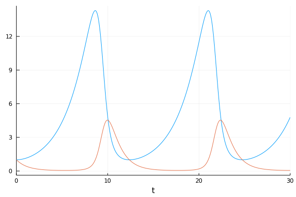

So, our linear model will be:

\(g \sim Distribution\_to\_be\_proposed()\) \(\mu[i] = g*\frac{t_{f}^2[i]}{2}\) \(\Delta x[i]= Normal(\mu[i],\sigma^2)\)

Where \(g\) has a distribution we will propose next. The first distribution we are going to propose is a uniform distribution for g, between the values of 0 and 10

begin
using Turing
using StatsPlots
plot(Uniform(0,10),xlim=(-1,11), ylim=(0,0.2), legend=false, fill=(0, .5,:lightblue))
title!("Uniform prior distribution for g")
xlabel!("g_mars")
ylabel!("Probability")
end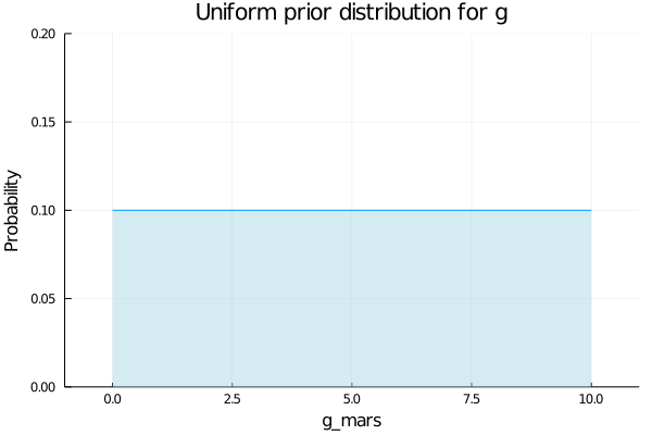

Now we define the model in Turing and sample from the posterior distribution.

begin
@model gravity_uniform(t_final, x_final, θ) = begin
    # The number of observations.
    g ~ Uniform(0,10)
    μ = g .* (t_final.*t_final./2)
        
    N = length(t_final)
    for n in 1:N
            x_final[n] ~ Normal(μ[n], 10)
        end
end;
end

begin
iterations = 10000
ϵ = 0.05
τ = 10
end;

begin
θ = 45
chain_uniform = sample(gravity_uniform(t_measured, Δx_measured, θ), HMC(ϵ, τ), iterations, progress=false);
end;

Plotting the posterior distribution for p we that the values are mostly between 2 and 5, with the maximun near 3,8. Can we narrow the values we obtain?

begin
    histogram(chain_uniform[:g], xlim=[1,6], legend=false, normalized=true)
    xlabel!("g_mars")
    title!("Posterior distribution for g with uniform distribution")
end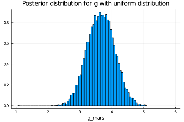

As a second obtion, we can propose a Gaussian distribution instead of a uniforn distribution for \(g\), like the one shown below, with a mean of 5 and a variance of 2, and let the model update its beliefs with the points we have.

begin
plot(Normal(5,2), legend=false, fill=(0, .5,:lightblue))
title!("Normal prior distribution for g")
xlabel!("g_mars")
ylabel!("Probability")
end

We define then the model with a gaussian distribution as a prior for \(g\):

begin
@model gravity_normal(t_final, x_final, θ) = begin
    # The number of observations.
    N = length(t_final)
    g ~ Normal(6,2)
    μ = g .* (t_final.*t_final./2)
        
    for n in 1:N
            x_final[n] ~ Normal(μ[n], 3)
        end
end;
end

Now we sample values from the posterior distribution and plot and histogram with the values obtained:

begin
chain_normal = sample(gravity_normal(t_measured, Δx_measured, θ), HMC(ϵ, τ), iterations, progress=false);
end;

begin
    histogram(chain_normal[:g], xlim=[3,4.5],legend=false, normalized=true)
    xlabel!("g_mars")
    title!("Posterior distribution for g with Normal distribution")

end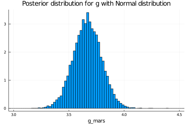

We see that the plausible values for the gravity have a clear center in 3.7 and now the distribution is narrower, that’s good, but we can do better.

If we observe the prior distribution proposed of \(g\), we see that some values are negative, which has no sense because if that would the case when you trow the stone, it would go up and up, escaping from the planet.

We propose then a new model for not allowing the negative values to happen. The distribution we are interested in is a LogNormal distribution. In the plot below is the prior distribution for g, a LogNormal distribution with mean 1.5 and variance of 0.5.

begin
plot(LogNormal(1,0.5), xlim=(0,10), legend=false, fill=(0, .5,:lightblue))
title!("Prior LogNormal Distribution for g")
ylabel!("Probability")
xlabel!("g")
end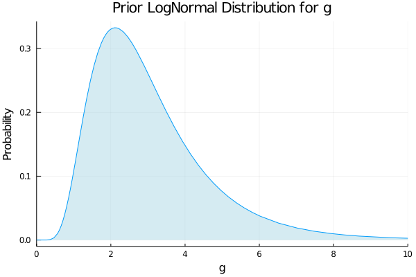

The model gravity_lognormal defined below has now a LogNormal prior. We sample the posterior distribution after updating with the data measured.

begin
@model gravity_lognormal(t_final, x_final, θ) = begin
    # The number of observations.
    N = length(t_final)
    g ~ LogNormal(0.5,0.5)
    μ = g .* (t_final.*t_final./2)
    for n in 1:N
            x_final[n] ~ Normal(μ[n], 3)
    end
end;
end

begin
chain_lognormal = sample(gravity_lognormal(t_measured, Δx_measured, θ), HMC(ϵ, τ), iterations, progress=false);
end;

begin
    histogram(chain_lognormal[:g], xlim=[3,4.5], legend=false, normalized=true)
    xlabel!("g_mars")
    title!("Posterior distribution for g with LogNormal distribution")

end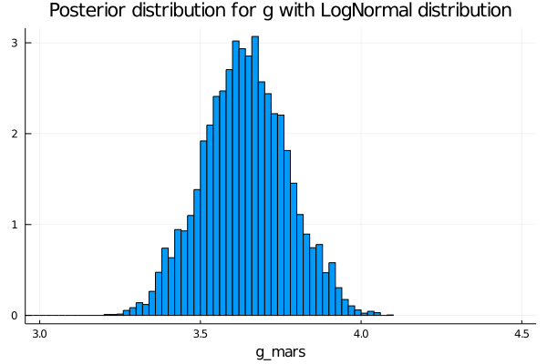

6.2 Optimizing the throwing angle

Now that we have a good understanding of the equations and the overall problem, we are going to add some difficulties and we will loosen a constrain we have imposed: Suppose that the device employed to measure the angle has an error of 15°, no matter the angle.

We want to know what are the most convenient angle to do the experiment and to measure or if it doesn’t matter.

To do the analysis we need to see how the angle influence the computation of \(g\), so solving the equation for \(g\) we have:

\(g = \frac{2*tg(\theta)*\Delta x}{t^{2}_f}\)

We can plot then the tangent of θ, with and error of 15° and see what is its maximum and minimun value:

begin
angles = 0:0.1:70
error = 15/2
μ = tan.(deg2rad.(angles))
ribbon = tan.(deg2rad.(angles .+ error)) - μ
plot(angles, μ, ribbon=ribbon, color="lightblue", legend=false)
ylabel!("tan(θ)")
xlabel!("θ [deg]")
title!("tan(θ) and its error")
end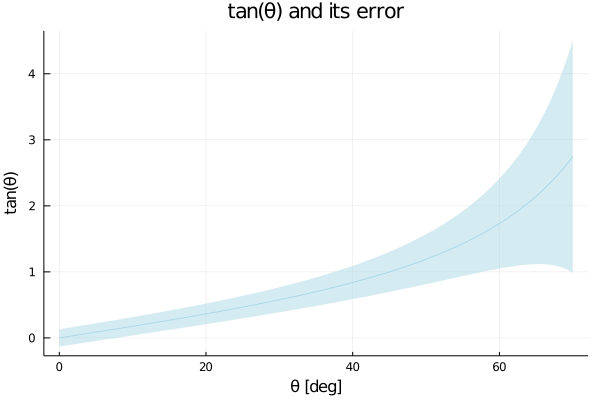

But we don’t care about the absolute value of the error, we want the relavite error, so plotting the percentual error we have:

begin
er= tan.(deg2rad.(angles .+ error)) .- tan.(deg2rad.(angles .- error))
perc_error = er .* 100 ./ μ
plot(angles, er .* 100 ./ μ, xlim=(5,70), ylim=(0,200), color="lightblue", legend=true, lw=3, label="Percentual error")
vline!([angles[findfirst(x->x==minimum(perc_error), perc_error)]], lw=3, label="Minimum error")
ylabel!("Δtan(θ)/θ")
xlabel!("θ [deg]")
title!("Percentual error")
end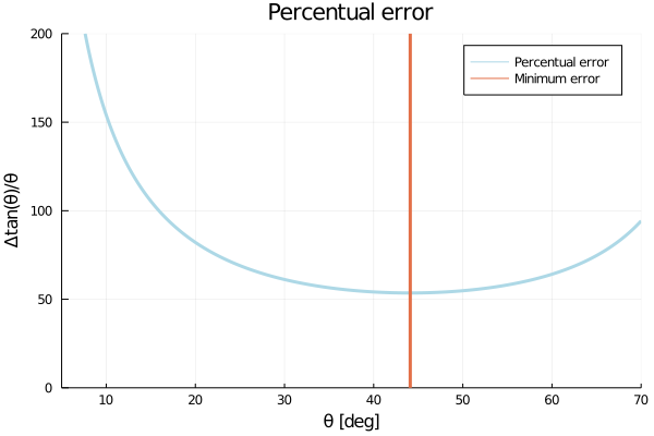

So, now we see that the lowest percentual error is obtained when we work in angles near 45°, so we are good to go and we can use the data we measured adding the error in the angle. We now define the new model, where we include an uncertainty in the angle. We propose an uniform prior for the angle centered at 45°, the angle we think the measurement was done.

begin
@model gravity_angle_uniform(t_final, x_final, θ) = begin
    # The number of observations.
    error = 15
    angle ~ Uniform(45-error/2, 45 + error/2)
    g ~ LogNormal(log(4),0.3)
    μ = g .* (t_final.*t_final./(2 * tan.(deg2rad(angle))))
        
    N = length(t_final)
    for n in 1:N
            x_final[n] ~ Normal(μ[n], 10)
        end
end;
end

begin
chain_uniform_angle = sample(gravity_angle_uniform(t_measured, Δx_measured, θ), HMC(ϵ, τ), iterations, progress=false);
end;

begin
    histogram(chain_uniform_angle[:g], legend=false, normalized=true)
    xlabel!("g_mars")
    ylabel!("Probability")
    title!("Posterior distribution for g, including uncertainty in the angle")
end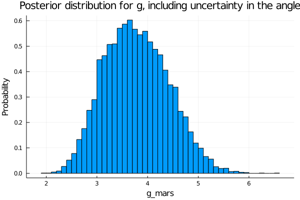

6.2.1 Calculating the escape velocity

Now that we have calculated the gravity, we are going to calculate the escape velocity.

What data do we have until now?

we know from the begining that:

\(R_{Earth}\approxeq 2R_{Mars}\) \(g_{Earth}\approxeq 9.8\)

and we have also computed the distribution of the plausible values of \(g_{Mars}\).

So, replacing them in the equation of the escape velocity:

\(\frac{v_{Mars}}{v_{Earth}} =\sqrt{\frac{g_{Mars}*R_{Mars}}{g_{Earth}*R_{Earth}}}\)

so,

\(\frac{v_{Mars}}{11} =\sqrt{\frac{g_{Mars}*2*\cancel{R_{Mars}}}{9.8*\cancel{R_{Mars}}}} \qquad \left[\frac{km}{s} \right]\)

\(v_{Mars} =11 * \sqrt{\frac{g_{Mars}}{9.8*2}} \qquad \left[\frac{km}{s} \right]\)

begin
    v = 11 .* sqrt.(chain_uniform_angle[:g] ./ (9.8*2))
    histogram(v, legend=false, normalized=true)
    title!("Escape velocity from Mars")
    xlabel!("Escape Velocity of Mars [km/s]")
    ylabel!("Probability")
    
end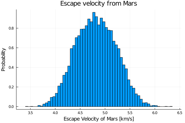

Finally, we obtained the escape velocity scape from Mars.

6.3 Summary

In this chapter we had to find the escape velocity from Mars. To solve this problem, we first needed to find the gravity of Mars, so we started with a physical description of the problem and concluded that by measuring the distance and time of a rock throw plus some Bayesian analysis we could infer the gravity of Mars.

Then we created a simple probabilistic model, with the prior probability set to a uniform distribution and the likelihood to a normal distribution. We sampled the model and obtained our first posterior probability. We repeated this process two more times, changing the prior distribution of the model for more accurate ones, first with a normal distribution and then with a logarithmic one.

Finally, we used the gravity we inferred to calculate the escape velocity from Mars.

6.4 Give us feedback

This book is currently in a beta version. We are looking forward to getting feedback and criticism:

• Submit a GitHub issue here.
• Mail us to martina.cantaro@lambdaclass.com

Thank you!